Interactive online versions:
Validation of non-Spin-Flip scattering with gepore.f
We can check a simple magnetic model \((\vec M \parallel \vec H)\) with no spin-flip scattering against:
gepore.f as written directly in the PNR book chapter [1]
gepore_zeeman.f (a slightly modified version of gepore.f that includes the Zeeman effect)
refl1d using the magnetic calculation kernel
refl1d using the unpolarized calculation kernel twice, with
\(\rho_{++} = \rho_N + \rho_M\)
\(\rho_{--} = \rho_N - \rho_M\)
We are using the Refl1D geometry convention where \(\text{Aguide} = 270^\circ, \theta_M = 270^\circ\) corresponds to an in-plane magnetic field with \(\vec M \parallel \vec H\). The sample will be a magnetic layer on a non-magnetic substrate, with a non-magnetic cap layer
[1] Majkrzak, C., O’Donovan, K. & Berk, N. (2006). Neutron Scattering from Magnetic Materials, edited by T. Chatterji, pp. 397–471. Amsterdam: Elsevier Science.
[1]:
# Install refl1d if it is not already installed
try:
    import refl1d
except ImportError:
    %pip install -q "refl1d @ git+https://github.com/reflectometry/refl1d"
    import refl1d
[2]:
import numpy as np
from refl1d.validation.gepore_runner import GeporeRunner

# start a GeporeRunner instance

runner = GeporeRunner()

QS = 0.001  # start value of Q
DQ = 0.0004  # step size in Q
NQ = 80  # number of Q points
Qz = np.arange(NQ) * DQ + QS
Define the sample as a list of layers:
label |
thickness (A) |
\(\text{SLD}_N\) \((10^{-6}A)\) |
\(\text{SLD}_M\) \((10^{-6}A)\) |
\(\theta_{M}\) \((\text{degrees})\) |
|---|---|---|---|---|
vacuum |
0 |
0.0 |
0.0 |
270 |
mag. layer |
1000 |
8.0 |
2.0 |
270 |
cap layer |
500 |
5.0 |
0.0 |
270 |
substrate |
0 |
2.0 |
0.0 |
270 |
[3]:
Aguide = 270.0  # guide field in sample plane
layers = [
    # depth rho rhoM thetaM phiM
    [0, 0.0, 0.0, 270, 0],
    [1000, 8.0, 2.0, 270, 0.0],
    [500, 5.0, 0.0, 270, 0.0],
    [0, 2.0, 0.0, 270, 0.0],
]
depth, rhoN, rhoM, thetaM, phiM = list(zip(*layers))
applied field, in Tesla, shouldn’t matter for this calculation
[4]:
H = 0.5
Calculating with gepore.f
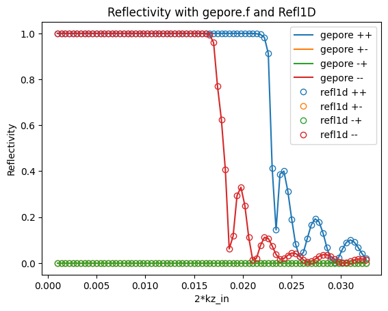
The reflectivities are returned from gepore.f in the order \((r_g^{++}, r_g^{+-}, r_g^{-+}, r_g^{--})\)
NOTE we use a value of \(\text{EPS} = -\text{Aguide}\)
[5]:
EPS = -Aguide
rg = runner.run(layers, QS, DQ, NQ, EPS, H, zeeman_corrections=False)
Rg = [np.abs(r) ** 2 for r in rg]
Calculating with the modified gepore_zeeman.f
A version of the original gepore.f that includes Zeeman energy corrections
[6]:
rgz = runner.run(layers, QS, DQ, NQ, EPS, H, zeeman_corrections=True)
Rgz = [np.abs(r) ** 2 for r in rgz]
Calculating reflectivity using Refl1D
magnetic_amplitude returns cross-sections in order \((r_1^{--}, r_1^{-+}, r_1^{+-}, r_1^{++})\), so we need to reverse them here to compare to gepore outputs
[7]:
from refl1d.sample.reflectivity import magnetic_amplitude, reflectivity_amplitude

r1 = magnetic_amplitude(Qz / 2, depth, rhoN, 0, rhoM, thetaM, 0, Aguide, H)
R1 = np.abs(r1[::-1]) ** 2
Calculating unpolarized reflectivity, with rhoN + rhoM and rhoN - rhoM
[8]:
rho_plus = np.array(rhoN) + np.array(rhoM)
rho_minus = np.array(rhoN) - np.array(rhoM)
sf = np.zeros_like(R1[0])
rnsf = (
    reflectivity_amplitude(Qz / 2, depth, rho_plus, 0, 0, None),
    sf,
    sf,
    reflectivity_amplitude(Qz / 2, depth, rho_minus, 0, 0, None),
)
Rnsf = [np.abs(r) ** 2 for r in rnsf]
Plots
[9]:
from matplotlib import pyplot as plt
[10]:
fig = plt.figure()
ax = fig.add_subplot(111)
xs_labels = ["++", "+-", "-+", "--"]
for i, label in enumerate(xs_labels):
    ax.plot(Qz, Rg[i], label=f"gepore {label}")
ax.set_prop_cycle(None)
for i, label in enumerate(xs_labels):
    ax.plot(Qz, R1[i], "o", label=f"refl1d {label}", fillstyle="none")
ax.set_ylabel("Reflectivity")
ax.set_xlabel("2*kz_in")
ax.set_title("Reflectivity with gepore.f and Refl1D")
ax.legend()
[10]:
<matplotlib.legend.Legend at 0x7f849735e6f0>

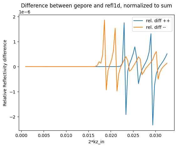
The differences between the two reflectivity outputs are small, and are likely due to differences in the numerical implementation of the reflectivity calculation. Here is a plot of the differences:
[11]:
fig = plt.figure()
ax = fig.add_subplot(111)
xs_labels = ["++", "+-", "-+", "--"]
for i, label in enumerate(xs_labels):
    if not i == 1 and not i == 2:  # skip +- and -+
        ax.plot(Qz, 2 * (Rg[i] - R1[i]) / np.abs(Rg[i] + R1[i]), label=f"rel. diff {label}")
ax.set_ylabel("Relative Reflectivity difference")
ax.set_xlabel("2*kz_in")
ax.set_title("Difference between gepore and refl1d, normalized to sum")
ax.legend()
[11]:
<matplotlib.legend.Legend at 0x7f84971553d0>

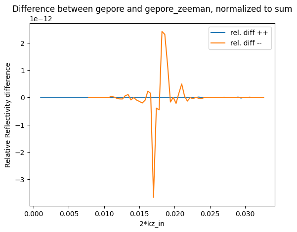
[12]:
fig = plt.figure()
ax = fig.add_subplot(111)

for i, label in enumerate(xs_labels):
    if not i == 1 and not i == 2:  # skip +- and -+
        ax.plot(Qz, 2 * (Rgz[i] - Rg[i]) / np.abs(Rgz[i] + Rg[i]), label=f"rel. diff {label}")
ax.set_ylabel("Relative Reflectivity difference")
ax.set_xlabel("2*kz_in")
ax.set_title("Difference between gepore and gepore_zeeman, normalized to sum")
ax.legend()
[12]:
<matplotlib.legend.Legend at 0x7f849401ff50>

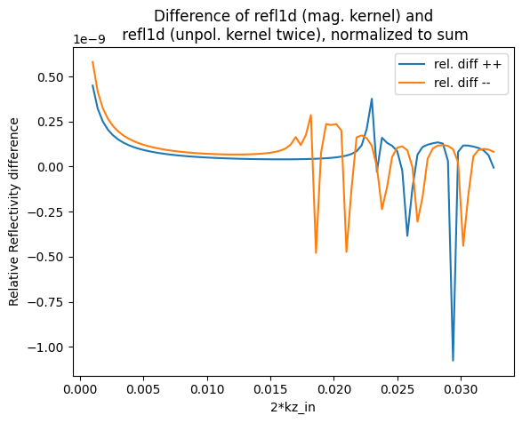
[13]:
fig = plt.figure()
ax = fig.add_subplot(111)
xs_labels = ["++", "+-", "-+", "--"]
for i, label in enumerate(xs_labels):
    if not i == 1 and not i == 2:  # skip +- and -+
        ax.plot(Qz, 2 * (Rnsf[i] - R1[i]) / np.abs(Rnsf[i] + R1[i]), label=f"rel. diff {label}")
ax.set_ylabel("Relative Reflectivity difference")
ax.set_xlabel("2*kz_in")
ax.set_title("Difference of refl1d (mag. kernel) and\n refl1d (unpol. kernel twice), normalized to sum")
ax.legend()
[13]:
<matplotlib.legend.Legend at 0x7f849718d6d0>

[ ]: